Training HNNs without backpropagation

Hamiltonian neural networks (HNNs) ¹ are a smart way to incorporate physical knowledge into neural networks. In this post we will dive into the main ideas behind our paper² and talk about what is exciting in this line of work! If you are not familiar with HNNs or sampling neural networks I hope this post also gives you an intuition behind their concepts and which problems they address. This post also contains code examples that I encourage you to code along and have fun! You can find the code in notebooks as reference. Note that the code provided here is for explanation purposes, you can checkout the code link below to reproduce the experiments from the paper.

Paper Code Poster Video

TLDR

We have trained HNNs by sampling the hidden layer parameters using data-agnostic and data-driven sampling methods and solving a linear system to fit the last linear layer parameters. The linear equation incorporates Hamilton's equations by design, therefore maintains HNN properties like energy conservation. We have also evaluated different algorithms for the sampling part and compared the performance of the sampled HNNs against iteratively (gradient-descent-based) trained HNNs. We have seen very accurate approximations from the sampled HNNs compared to traditionally trained HNNs, and the data-driven sampling is superior to data-agnostic sampling when the target function has large gradients or large input domain in our numerical experiments.

Introduction: Introduces Hamiltonian systems and how to solve them using numeric methods with examples.

Method: Explains the key idea of utilizing sampling algorithms for training HNNs.

Results & Discussion: Shows some of our results from the paper and concludes this post.

For detailed explanation you can check out the sections you find interesting from the table of contents.

Introduction

Can we quickly train accurate HNNs?

Our recent paper, “Training Hamiltonian neural networks without backpropagation”, introduces an approach that does just that. By leveraging data-driven methods, we achieve both high accuracy and high speed in training HNNs. Here’s a deep dive into the ideas, methods and results that make this work so exciting.

Hamiltonian systems

Hamiltonian systems are the heart of modeling physical phenomena from pendulum to planetary motion. And there is more, Hamiltonian systems are not just encountered in physics, there are Hamiltonian systems and their analysis in economics (Pontryagin’s maximum principle), biology (Lotka-Volterra), and many more. What’s more exciting is we can model these systems directly from data, e.g. by using neural networks as we will see in a moment. This provides us a way to learn these systems (and solve them) without knowing the underlying equations of motion.

At the core, Hamiltonian systems are defined by a scalar valued Hamiltonian function which maps the state of the system into a conserved quantity (e.g. energy in mechanical systems). Using Hamilton’s equations ³ (and knowing the Hamiltonian function) we can retrieve the equations of motion of the system. Therefore, we are usually interested in knowing (or approximating) Hamiltonian functions.

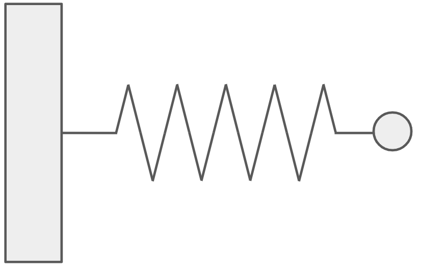
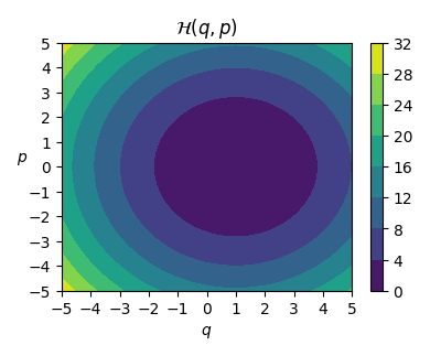
We can approximate a Hamiltonian function to learn a Hamiltonian system.

Now, let’s focus on the goal of approximating Hamiltonian functions, that is, functions that describe equations of motions to many dynamical systems. Let’s inspect one simple example Hamiltonian system from mechanics: Mass-spring system, where the Hamiltonian function value describes the conserved total ’energy’ of the system.

Click to see the code

import numpy as np
import matplotlib as mpl
import matplotlib.pyplot as plt

GOLDEN_RATIO = (1 + 5**0.5) / 2 # for plotting

def spring_hamiltonian(x):
    # H(q,p) = 1/(2m) * p^2 + k/2 (q-L)^2
    # with Mass m=1, Spring constant k=1, natural spring length L=1
    # H(q,p) = 0.5 * p^2 + 0.5 * (q-1)^2
    q, p = np.split(x, 2, axis=-1)
    return 0.5 * p**2 + 0.5 * (q-1)**2

# visualize system
q = np.linspace(-5, 5, 1000)
p = np.linspace(-5, 5, 1000)
qs, ps = np.meshgrid(q, p, indexing="ij")
x = np.column_stack([qs.flatten(), ps.flatten()])
Hx = spring_hamiltonian(x)


fig, ((ax0)) = plt.subplots(1, 1, figsize=(4, 2*GOLDEN_RATIO), dpi=100)
im = ax0.contourf(q, p, Hx.reshape(q.size, p.size).T)
fig.colorbar(im, ax=ax0)
ax0.set_title(r"$\mathcal{H}(q,p)$")
ax0.set_xlabel(r"$q$")
ax0.set_ylabel(r"$p$", rotation=0)
ax0.set_xticks(list(range(-5, 6)))
ax0.set_yticks(list(range(-5, 6)))
fig.tight_layout()
fig.savefig("../../static/images/posts/training-hnns-without-backprop/mass-spring-true-hamil.png")

A mass is connected to a horizontal spring.

Periodic Hamiltonian function of the mass spring system is visualized.

Left: Mass-spring system is visualized. Right: Its Hamiltonian function is plotted.

When the constants are set (see the code for details) we get the target function as: $$ \mathcal{H}(q,p) = \frac{p^2}{2} + \frac{(q-1)^2}{2}, $$ where $\mathcal{H}: \mathbb{R}^2 \rightarrow \mathbb{R}$ is the Hamiltonian function.

Usually we are interested in solving the system given an initial position $x_0 = (q_0, p_0)$. The equations of motion can be recovered using the Hamilton’s equations:

$$ \dot{q} = \partial \mathcal{H} / \partial p $$

and

$$ \dot{p} = -\partial \mathcal{H} / \partial q, $$

that is, we can recover $\dot{q} = \partial{q} / \partial{t}$ and $\dot{p} = \partial{p} / \partial{t}$ from the partial derivatives of the Hamiltonian function value w.r.t. $q$ and $p$, which describe the evolution of our system. What this means is, we can use the time derivatives to ‘solve’ the system for any given initial condition $x_0 = (q_0,p_0)$, e.g. by applying the forward Euler method to compute the next state of the system at $x_1 = (q_1,p_1) = (q_0 + \Delta t \cdot \dot{q}_0, p_0 + \Delta t \cdot \dot{p}_0)$ and continue this process until a trajectory $(x_0, x_1, \dots, x_N )$ is approximated.

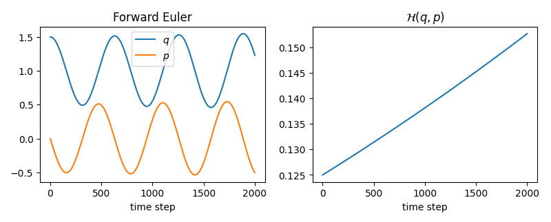
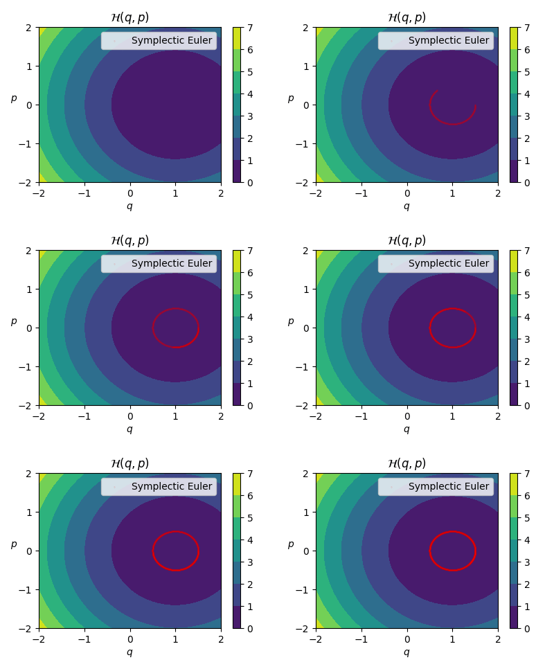
If we know the gradient of the Hamiltonian function we can retrieve the time derivatives of the position and momenta at any point using Hamilton’s equations.

Let’s approximate the trajectory for the initial state $x_0 = (1.5, 0)$ using forward Euler as it is quite straightforward to implement.

Click to see the code

def dH(x):
    """
    partial derivatives of H w.r.t. q and p
    dHdq = 0.5 * 2*(q-1) = q-1
    dHdp = 0.5 * 2*p = p
    returns the gradient dHdx = [dHdq, dHdp]
    """
    q, p = x[0], x[1]
    return np.array([q - 1, p])

def hamiltons_equations(dHdx):
    """
    returns time derivatives [dqdt, dpdt]
    using Hamilton's equations
    """
    dHdq, dHdp = dHdx[0], dHdx[1]
    q_dot, p_dot = dHdp, -dHdq
    return np.array([q_dot, p_dot])

def forward_euler(x, dt):
    """
    x_next = x_prev + dt * x_prev_dot
    """
    dHdx = dH(x)
    dxdt = hamiltons_equations(dHdx)

    return x + dt * dxdt

dt = 1e-2
traj_length = 2000
x_0 = np.array([1.5, 0.])

forward_euler_traj = [x_0]
for _ in range(traj_length-1):
    x = forward_euler_traj[-1]
    x_next = forward_euler(x, dt)
    forward_euler_traj.append(x_next)

forward_euler_traj = np.array(forward_euler_traj)
hamiltonian_values = spring_hamiltonian(forward_euler_traj)

fig, ((ax0, ax1)) = plt.subplots(1, 2, figsize=(8, 2*GOLDEN_RATIO), dpi=100)
ax0.plot(range(1, traj_length+1), forward_euler_traj[:,0], label=r"$q$")
ax0.plot(range(1, traj_length+1), forward_euler_traj[:,1], label=r"$p$")
ax0.set_title(r"Forward Euler")
ax0.set_xlabel(r"time step")
ax0.legend()
ax1.plot(range(1, traj_length+1), hamiltonian_values)
ax1.set_xlabel(r"time step")
ax1.set_title(r"$\mathcal{H}(q,p)$")
fig.tight_layout()
fig.savefig("../../static/images/posts/training-hnns-without-backprop/mass-spring-forward-euler.png")

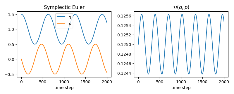
Forward Euler integration of the system is visualized from an initial point. Hamiltonian value is not conserved in the forward Euler integration.

Left: $q$ and $p$ values are plotted for each time step ($\Delta t = 10^{-2}$). Right: Hamiltonian value is plotted at each time step.

We notice that the Hamiltonian value (total energy of the system) diverges on the right plot. However, we did not ‘add’ or ‘remove’ energy (we are dealing with a closed system), so why does this happen? This is due to the forward Euler integration, which does not have conserving properties. When dealing with Hamiltonian systems we should therefore resort to symplectic integrators with conserving properties. The flow map (evolution operator in our case) of a Hamiltonian system is a symplectic map. Let’s try the symplectic Euler integration method and see the difference.

Click to see the code

def symplectic_euler(x, dt):
    """
    mass-spring is a separable system:
    - q_dot depends only on p,  (q_dot =  dHdp(_, p) = p)
    - p_dot depends only on q.  (p_dot = -dHdq(q, _) = q-1)

    q_next = q_prev + dt * q_dot(p_prev)
    p_next = p_prev + dt * p_dot(q_next)

    Uses x_next (p_dot only depends on q_next)
    in the update for p_next
    """
    dHdx = dH(x)
    dxdt = hamiltons_equations(dHdx)
    dqdt = dxdt[0]

    # update q
    q, p = x[0], x[1]
    q_next = q + dt * dqdt

    dHdx_next = dH(np.array([q_next, p]))
    dxdt_next = hamiltons_equations(dHdx_next)
    dpdt_next = dxdt_next[1]

    # update p
    p_next = p + dt * dpdt_next

    return np.array([q_next, p_next])

dt = 1e-2
traj_length = 2000
x_0 = np.array([1.5, 0.])

symplectic_euler_traj = [x_0]
for _ in range(traj_length-1):
    x = symplectic_euler_traj[-1]
    x_next = symplectic_euler(x, dt)
    symplectic_euler_traj.append(x_next)

symplectic_euler_traj = np.array(symplectic_euler_traj)
hamiltonian_values = spring_hamiltonian(symplectic_euler_traj)
    fig, ((ax0, ax1)) = plt.subplots(1, 2, figsize=(8, 2*GOLDEN_RATIO), dpi=100)
ax0.plot(range(1, traj_length+1), symplectic_euler_traj[:,0], label=r"$q$")
ax0.plot(range(1, traj_length+1), symplectic_euler_traj[:,1], label=r"$p$")
ax0.set_title(r"Symplectic Euler")
ax0.set_xlabel(r"time step")
ax0.legend()
ax1.plot(range(1, traj_length+1), hamiltonian_values)
ax1.set_xlabel(r"time step")
ax1.set_title(r"$\mathcal{H}(q,p)$")
fig.tight_layout()
fig.savefig("../../static/images/posts/training-hnns-without-backprop/mass-spring-symplectic-euler.png")

Symplectic Euler integration of the system is visualized from an intial point, where we see the conserving property of the symplectic integrator, that is, the Hamiltonian value is conserved.

Left: $q$ and $p$ values are plotted for each time step ($\Delta t = 10^{-2}$). Right: Hamiltonian value is plotted at each time step.

With this we also make a sanity check of our implementation and see the harmonic – oscillating motion of the harmonic mass-spring system.

Great! Now we have a system that we can analytically integrate using the true Hamiltonian function and approximate trajectories given any initial state of the system. We can even create animations.

Click to see the code

from IPython.display import HTML
from matplotlib.animation import FuncAnimation

# focused visualization of the system
q = np.linspace(-2, 2, 1000)
p = np.linspace(-2, 2, 1000)
qs, ps = np.meshgrid(q, p, indexing="ij")
x = np.column_stack([qs.flatten(), ps.flatten()])
Hx = spring_hamiltonian(x)

fig, ((ax0)) = plt.subplots(1, 1, figsize=(4, 2*GOLDEN_RATIO), dpi=100)
im = ax0.contourf(q, p, Hx.reshape(q.size, p.size).T)
fig.colorbar(im, ax=ax0)
ax0.set_title(r"$\mathcal{H}(q,p)$")
ax0.set_xlabel(r"$q$")
ax0.set_ylabel(r"$p$", rotation=0)
ax0.set_xticks(list(range(-2, 3)))
ax0.set_yticks(list(range(-2, 3)))

# plot params
scatter_size = 1.5
color = "red"
alpha = 0.05

scat = ax0.scatter(symplectic_euler_traj[0,0], symplectic_euler_traj[0,1], c=color, s=scatter_size, label="Symplectic Euler", alpha=alpha)
ax0.legend()
fig.tight_layout()

num_frames = 50
batch_size = int(len(symplectic_euler_traj) / 50)

def update(frame):
    idx = frame * batch_size
    scat.set_offsets(symplectic_euler_traj[:idx])
    return scat

ani = FuncAnimation(fig=fig, func=update, frames=num_frames, interval=50)
plt.close()
ani.save("../../static/images/posts/training-hnns-without-backprop/mass-spring-integration-anim.gif", "imagemagick")
HTML(ani.to_jshtml())

Symplectic Euler approximated trajectory is animated. $\Delta t = 10^{-2}$, for 2000 time steps.

Visualizing physical systems by creating plots and animations is in my opinion very interesting and fun to play around and luckily Hamiltonian systems gives us a broad range of plotting opportunities.

Now let’s focus on the questions we might be asking at this point:

How do we learn the Hamiltonian function and query its gradient at any point?

Can we make the same plots and observations using trained neural networks?

Given a dataset $\lbrace q_i, p_i, \dot{q}_i, \dot{p}_i \rbrace _{i=1}^{K}$ we could be interested in modeling the single pendulum system. We could model this system using a neural network as an ODE-Net that takes $q$ and $p$ as input and outputs $\dot{q}$ and $\dot{p}$ directly. This way, after training the model we should be able to query the time derivative information at any state of the system, and use an integrator to approximate the evolution of the system given any initial condition. However, by doing so, we neglect the Hamiltonian function and the underlying physics: Hamilton’s equations! Recent work (HNNs) compared HNNs with plain ODE-Nets. Let’s see how HNNs are traditionally constructed in the following.

Hamiltonian neural networks

We re-iterate our question to:

How can we model the Hamiltonian function from data and retrieve its gradient?

Hamiltonian architecture is visualized, input is position and momentum and model outputs Hamiltonian value. Using auto-differentiation and Hamilton's equations we recover the time derivatives of the position and momentum.

HNN architecture is visualized.

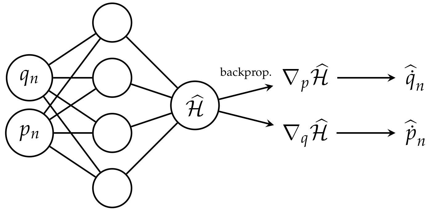
HNNs directly approximate the Hamiltonian function from data and use automatic differentiation to retrieve the partial derivatives of the model w.r.t to its inputs $q$ and $p$ at any state of the system. They are also trained with a custom loss function incorporating the Hamilton’s equations:

$$ \mathcal{L} = \bigg\lVert \frac{\partial \widehat{\mathcal{H}}}{\partial p} - \frac{\partial q}{\partial t} \bigg\rVert_2 + \bigg\lVert \frac{\partial \widehat{\mathcal{H}}}{\partial q} + \frac{\partial p}{\partial t} \bigg\rVert_2, $$

where $\widehat{\mathcal{H}}$ is parameterized by a neural network, and it approximates the target Hamiltonian function. After training, HNNs can retrieve both the conserved state of the system (the Hamiltonian) and the time derivatives of $q$ and $p$ by applying the Hamilton’s equations on the gradients of the model’s output (retrieved through automatic differentiation).

HNNs studies the question above, and can directly use the Hamilton’s equations thus incorporating our physical knowledge into the approximation! Let’s train an HNN to approximate the mass-spring Hamiltonian function.

Click to see the code for imports and HNN training constants

import os
import torch
import torch.nn as nn
from torch.optim import Adam
from time import time

# For ADAM training
SEED_TORCH = 91234
DEVICE = 'cuda' # choose accordingly to our hardware 'cpu' or 'cuda'
NUM_TRAIN_STEPS = 20000
BATCH_SIZE = 512
LEARNING_RATE = 5e-4
WEIGHT_DECAY = 1e-13
NUM_HIDDEN_NEURONS = 1000
torch.manual_seed(SEED_TORCH)
torch.set_default_dtype(torch.float64)
torch.set_num_threads(os.cpu_count())

Click to see the code for data generation

import numpy as np

# For generating data
SEED_DATA = 752123
RNG = np.random.default_rng(SEED_DATA)
NUM_POINTS = 10000
TRAIN_SPLIT = 0.8 # means we use 80% of the data for training
                  #              20% of the data for testing

def dxdt(x):
    # gradient of the mass-spring Hamiltonian w.r.t. input:
    # returns dx/dt = (dq/dt, dp/dt) (time derivative of input)
    q, p = np.split(x, 2, axis=-1)
    dHdq, dHdp = q-1, p
    # Hamilton's equations
    dqdt, dpdt = dHdp, -dHdq
    return np.column_stack([dqdt.flatten(), dpdt.flatten()])

qs = RNG.uniform(low=-5, high=5, size=(NUM_POINTS))
ps = RNG.uniform(low=-5, high=5, size=(NUM_POINTS))
x = np.column_stack([qs.flatten(), ps.flatten()])

# Shuffle
idx = RNG.permutation(x.shape[0])
x = x[idx]

# Train/Test split
split_idx = int(x.shape[0] * TRAIN_SPLIT)
x_train, x_test = x[:split_idx], x[split_idx:]
x_dot_train = dxdt(x_train)

# We assume we know the Hamiltonian at one point
# to correctly set the integration constant.
# Here we assumed we know where 'energy' is zero:
# -> At the equilibrium.
x0_train = np.array([[1.,0.]])
H0_train = spring_hamiltonian(x0_train) # equals zero

# Ground truths
y_train = spring_hamiltonian(x_train)
y_test = spring_hamiltonian(x_test)

Click to see the code for HNN implementation

class MLP(nn.Module):
    def __init__(self, input_dim, hidden_dim, output_dim):
        super(MLP, self).__init__()

        self.flatten = nn.Flatten()
        self.linear1 = nn.Linear(input_dim, hidden_dim)
        self.activation = nn.Tanh()
        self.linear2 = nn.Linear(hidden_dim, output_dim)

    def init_params(self):
        nn.init.xavier_normal_(self.linear1.weight)
        nn.init.zeros_(self.linear1.bias)

        nn.init.xavier_normal_(self.linear2.weight)
        nn.init.zeros_(self.linear2.bias)

    def forward(self, x):
        x = self.flatten(x)

        # dense layer
        x = self.linear1(x)
        x = self.activation(x)

        # linear layer
        x = self.linear2(x)

        return x

class HNN(nn.Module):
    def __init__(self, input_dim, hidden_dim):
        super(HNN, self).__init__()

        self.mlp = MLP(input_dim, hidden_dim, 1)

    def init_params(self):
        self.mlp.init_params()

    def forward(self, x):
        hamil = self.mlp(x)

        # Auto-diff
        hamil_dx = torch.autograd.grad(hamil.sum(), x, create_graph=True)[0]
        hamil_dq, hamil_dp = torch.split(hamil_dx, hamil_dx.shape[1] // 2, dim=1)

        # Hamilton's equations
        q_dot = hamil_dp
        p_dot = -hamil_dq

        return torch.cat((q_dot, p_dot), dim=1)

Click to see the code for optimization loop

def get_batch(x, step, batch_size, requires_grad=False):
    x_len, _ = x.shape
    i_begin = (step * batch_size) % x_len
    x_batch = x[i_begin:i_begin + batch_size, :]
    return torch.tensor(x_batch, requires_grad=requires_grad, device=DEVICE)

def train_step(model, optim, x, x_dot_true, idx_step):
    x_dot_pred = model.forward(x)
    loss = (x_dot_true - x_dot_pred).pow(2).mean()
    loss.backward(); optim.step(); optim.zero_grad()

    if idx_step % 1000 == 0:
        print(f"-> Loss at step {idx_step}\t:\t{loss}")

    return loss.item()

def adam_train(model, x_train, x_dot_train, x0, H0):
    model.to(DEVICE); model.train(); model.init_params()
    optim = Adam(model.parameters(), lr=LEARNING_RATE, weight_decay=WEIGHT_DECAY)
    train_losses = []

    print("Step No. : Loss (Squared L2 Error)")
    for idx_step in range(NUM_TRAIN_STEPS):
        x = get_batch(x_train, idx_step, BATCH_SIZE, requires_grad=True)
        x_dot_true = get_batch(x_dot_train, idx_step, BATCH_SIZE)
        loss = train_step(model, optim, x, x_dot_true, idx_step)
        train_losses.append(loss)

    # fit integration constant
    x = get_batch(x0, 0, 1)
    Hx_true = get_batch(H0, 0, 1)

    # MLP inside HNN outputs H(x)
    Hx_pred = model.mlp(x)
    bias = Hx_true - (Hx_pred - model.mlp.linear2.bias)
    model.mlp.linear2.bias = torch.nn.Parameter(bias)

    model.cpu()
    return train_losses

hnn = HNN(2, NUM_HIDDEN_NEURONS)

t0 = time()
train_losses = adam_train(hnn, x_train, x_dot_train, x0_train, H0_train)
t1 = time()
print(f"ADAM Training took {(t1-t0):.2f} seconds")

Click to see the code for evaluation

fig, ((ax)) = plt.subplots(1, 1, figsize=(4, 2*GOLDEN_RATIO), dpi=100)
ax.plot(list(range(1, NUM_TRAIN_STEPS+1)), np.log10(train_losses))
ax.set_xlabel('Step')
ax.set_title(r'Train loss, $\log_{10}$ scale')
fig.tight_layout()
fig.savefig("../../static/images/posts/training-hnns-without-backprop/hnn-training-loss.png")

def rel_l2_error(y_true, y_pred):
    return np.sqrt(((y_true - y_pred)**2).sum()) / np.sqrt(((y_true)**2).sum())

y_train_pred = hnn.mlp(torch.tensor(x_train)).detach().numpy()
y_test_pred = hnn.mlp(torch.tensor(x_test)).detach().numpy()

hnn_train_error = rel_l2_error(y_train, y_train_pred)
hnn_test_error = rel_l2_error(y_test, y_test_pred)

print(f"HNN train error: {hnn_train_error:.2E}")
print(f"HNN test  error: {hnn_test_error:.2E}")

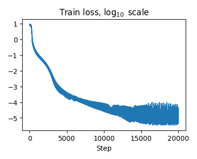
Training loss is plotted plateuing around -5 in log scale.

HNN training loss curve is plotted.

When using gradient-based optimizer (e.g. Adam) we have to define many hyperparameters such as NUM_TRAINING_STEPS, BATCH_SIZE, LEARNING_RATE, WEIGHT_DECAY, different weight initialization techniques if possible to see which works best, or learning rate scheduler parameters if there is one. And it is a very difficult task to tune these parameters and find the best parameters because the training itself takes usually quite a long time. On my laptop for example the training took about 220 seconds on CPUs (16 cores) and about 50 seconds on a GPU (NVIDIA RTX 3060 Mobile). And this is only for 8000 training points and 1000 hidden layer neurons. It usually gets more tedious when working with larger datasets and models. Our trained HNN could approximate the target Hamiltonian with high accuracy:

HNN train error: 1.55E-03
HNN test  error: 1.55E-03

and note that this is relative $L^2$ error.

HNNs are also used in many recent work with more complicated neural network architectures thus facing some challenges such as slow convergence due to the gradient-descent based iterative optimization of network parameters using backpropagation.

Can we bypass backpropagation?

Sampling

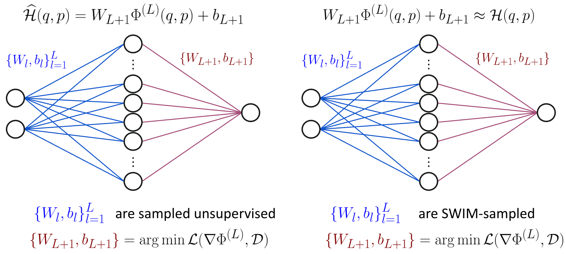
Sampling refers to ‘sampling the hidden layer parameters of (deep) neural networks’. In our work we focused on the following sampling algorithms:

Data-agnostic sampling – Extreme Learning Machine (ELM)
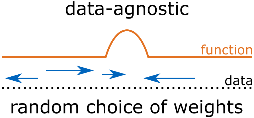
- samples the hidden layer parameters from fixed distributions: $\text{weight} \sim \mathcal{N}(0,1)$ and $\text{bias} \sim U(a,b)$ which means we are sampling all the weights and biases in the hidden layers using standard Gaussian and a fixed uniform distribution, respectively.
- Sampling of the hidden layer parameters are independent of observed data.
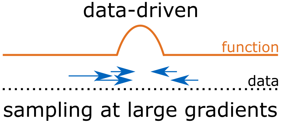
Data-driven sampling – Sample Where It Matters (SWIM)⁴
- samples the hidden layer parameters using the SWIM algorithm which constructs each weight-bias pair using a pair of data points picked from the data space.
- Sampling of the hidden layer parameters depend on the observed data.
- Sampling uses the gradient information from observed data to construct efficient weights (focus on where the function changes the most).

Data-agnostic sampling where weights are placed randomly

Data-driven sampling where weights are placed at large gradients

Data-agnostic and data-driven sampling of the weights are visualized [SWIM].

Can we utilize sampling to quickly train accurate HNNs?

Method

Sampling Hamiltonian neural networks

To make this concrete, here’s how we construct and train sampled HNNs:

First, sample the hidden layer parameters using any of the sampling algorithms explained above,
then solve a linear least squares problem that incorporates Hamilton’s equations for the final linear layer: $$(w^{\text{linear layer}}, b^{\text{linear layer}}) = \arg\min \mathcal{L}(\nabla \Phi, \mathcal{D}).$$

We can replace the backpropagation by analytically computing the gradients of hidden layer outputs.

$\Phi$ is the hidden layer output of our neural network. We use the differentiable activation function $\tanh$ and therefore can compute the analytical gradient w.r.t. the input. We denote it by $\nabla \Phi$. Finally, our loss term includes the observed time derivatives and incorporates the Hamilton’s equations. You can find it in more detail in our paper if you are interested how the linear system is defined exactly.

But how do we pick data pairs for the SWIM algorithm for the sampling step? Here we have the options

to pick the pairs uniformly: Uniform-SWIM (U-SWIM) or
pick the pairs at the large gradients: (SWIM).

How can we use the SWIM algorithm if it uses a supervised probability distribution?

The latter option is defined by a supervised probability distribution proportional to: $\frac{ \lVert \mathcal{H}(x^{(2)}) - \mathcal{H}(x^{(1)}) \rVert }{ \lVert x^{(2)} - x^{(1)} \rVert } $, that is, it puts more likelihood on the point pairs where the function changes more quickly (where the gradient is large). Unfortunately in real world data the Hamiltonian values (e.g. energy) is very hard to obtain. So our training set $\mathcal{D}$ does not contain the true function values, and thus this probability distribution is not available for us to use.

Use U-SWIM approximations in SWIM-sampling!

Approximate-SWIM sampling

Initial approximation is visualized on the left, which uses an unsupervised sampling algorithm and the Approximate-SWIM is visualized on the right which uses the initial approximation when sampling the pairs of points.

Left: Initial approximation using an unsupervised sampling algorithm. Right: Resample using the initial approximation with the propsed supervised probability distribution.

I gave the spoiler above: we can use an approximation instead for the SWIM algorithm, that is, we can use any approximation (in this work we used U-SWIM for the initial approximation) and then resample the hidden layer parameters using the SWIM algorithm and their proposed probability distribution. We called this version the Approximate-SWIM (A-SWIM). Let’s also see how we can implement sampled HNNs using the swimnetworks package. See the notebooks folder for the forked repository.

Click to see the code for imports and HNN sampling constants

from sklearn.pipeline import Pipeline
from swimnetworks.swimnetworks import Dense, Linear

SEED_MODEL = 91234 # to be used in the swimnetworks

# sampling parameters
RCOND = 1e-13
METHOD = "A-SWIM"

Click to see the code for Sampled-HNN implementation

class SampledMLP(nn.Module):
    def __init__(self, input_dim, hidden_dim, output_dim):
        super(SampledMLP, self).__init__()

        steps = [
            (
                "dense",
                Dense(
                    layer_width=NUM_HIDDEN_NEURONS,
                    activation="tanh",
                    elm_bias_start=-5.,
                    elm_bias_end=5.,
                    parameter_sampler="random",
                    sample_uniformly=True,
                    resample_duplicates=True,
                    random_seed=SEED_MODEL,
                )
            ),
            (
                "linear",
                Linear(layer_width=output_dim, regularization_scale=RCOND)
            )
        ]
        self.pipeline = Pipeline(steps)

    def forward(self, x):
        return self.pipeline.transform(x)

def tanh_grad(x):
    # analytical gradient of tanh
    return 1 - np.tanh(x)**2

class SampledHNN(nn.Module):
    def __init__(self, input_dim, hidden_dim):
        super(SampledHNN, self).__init__()

        self.mlp = SampledMLP(input_dim, hidden_dim, 1)

    def dense_grad(self, x):
        # Computes the gradient of dense_layer w.r.t. x
        dense_layer = self.mlp.pipeline[0]
        linear_layer = self.mlp.pipeline[-1]

        dense_layer.activation = tanh_grad
        dense_grad = dense_layer.transform(x)
        dense_layer.activation = np.tanh

        # computes dense_grad
        dense_grad = np.einsum('ij,kj->ikj', dense_grad, dense_layer.weights)

        return dense_grad

    def forward(self, x):
        # Compute the Hamiltonian gradient dHdx analytically
        # dense_grad * linear_weights
        dense_grad = self.dense_grad(x)
        linear_layer = self.mlp.pipeline[-1]

        # computes dHdx = dense_grad * linear_weights
        dHdx = (dense_grad @ linear_layer.weights).reshape(x.shape)

        dHdq, dHdp = np.split(dHdx, 2, axis=1)

        # Hamilton's Equations
        q_dot = dHdp
        p_dot = -dHdq

        return np.hstack((q_dot, p_dot))

Click to see the code for training sampled-HNNs

def sampling_train(model, x_train, x_dot_train, x0, H0, method):
    dense_layer = model.mlp.pipeline[0]
    linear_layer = model.mlp.pipeline[-1]

    if method == "ELM":
        dense_layer.parameter_sampler = "random"
    else:
        dense_layer.parameter_sampler = "tanh"

    dense_layer.__post_init__()

    # sample hidden layer parameters (unsupervised)
    dense_layer.fit(x_train)

    dense_grad = model.dense_grad(x_train)
    dense_x0 = dense_layer.transform(x0)
    params = solve_linear_system(dense_grad, dense_x0, x_dot_train, H0)

    # set linear layer weights and biases to the least-squres solution
    linear_layer.weights = params[:-1].reshape((-1, 1))
    linear_layer.biases = params[-1].reshape((1, 1))

    # re-sample supervised if Approximate SWIM
    if method == "A-SWIM":
        y_pred = model.mlp(x_train)

        # Sample using SWIM-proposed
        # data-pair picking probability
        dense_layer.sample_uniformly = False
        dense_layer.fit(x_train, y_pred)

        # retrain (solve least-squares) to fit
        # last linear layer parameters
        dense_grad = model.dense_grad(x_train)
        dense_x0 = dense_layer.transform(x0)
        params = solve_linear_system(dense_grad, dense_x0, x_dot_train, H0)

        linear_layer.weights = params[:-1].reshape((-1, 1))
        linear_layer.biases = params[-1].reshape((-1, 1))

def solve_linear_system(dense_grad, dense_x0, x_dot_train, H0):
    # construct linear system A * params = b
    dense_grad_q, dense_grad_p = np.split(dense_grad, 2, axis=1)

    # dof=degrees of freedom, for mass-spring it is 1
    (num_points, dof, hidden_size) = dense_grad_q.shape
    dense_grad_q = dense_grad_q.reshape(num_points*dof, hidden_size)
    dense_grad_p = dense_grad_p.reshape(num_points*dof, hidden_size)

    # Hamilton's Equations
    A = np.concatenate(( dense_grad_p, -dense_grad_q ), axis=0)
    A = np.concatenate(( A, dense_x0 ), axis=0)
    # For the bias term, add ones-column
    A = np.column_stack((A, np.concatenate(( np.zeros(A.shape[0] - 1), np.ones(1) ), axis=0) ))

    q_dot, p_dot = np.split(x_dot_train, 2, axis=1)
    b = np.concatenate((
        q_dot.ravel(),
        p_dot.ravel(),
        H0.ravel(),
    ))

    params = np.linalg.lstsq(A, b, rcond=RCOND)[0]
    # +1 because of linear layer bias (integration constant)
    return params.reshape(-1, 1) # final shape

METHOD = "A-SWIM"
sampled_hnn = SampledHNN(2, NUM_HIDDEN_NEURONS)
t0 = time()
sampling_train(sampled_hnn, x_train, x_dot_train, x0_train, H0_train, METHOD)
t1 = time()
print(f"Sampling training took {(t1-t0):.2f} seconds")

def rel_l2_error(y_true, y_pred):
    return np.sqrt(((y_true - y_pred)**2).sum()) / np.sqrt(((y_true)**2).sum())

y_train_pred = sampled_hnn.mlp(x_train)
y_test_pred = sampled_hnn.mlp(x_test)

hnn_train_error = rel_l2_error(y_train, y_train_pred)
hnn_test_error = rel_l2_error(y_test, y_test_pred)

print(f"- {METHOD}")
print(f"SampledHNN train error: {hnn_train_error:.2E}")
print(f"SampledHNN test  error: {hnn_test_error:.2E}")

METHOD = "ELM"
sampled_hnn = SampledHNN(2, NUM_HIDDEN_NEURONS)
t0 = time()
sampling_train(sampled_hnn, x_train, x_dot_train, x0_train, H0_train, METHOD)
t1 = time()
print(f"Sampling training took {(t1-t0):.2f} seconds")

y_train_pred = sampled_hnn.mlp(x_train)
y_test_pred = sampled_hnn.mlp(x_test)

hnn_train_error = rel_l2_error(y_train, y_train_pred)
hnn_test_error = rel_l2_error(y_test, y_test_pred)

print(f"- {METHOD}")
print(f"SampledHNN train error: {hnn_train_error:.2E}")
print(f"SampledHNN test  error: {hnn_test_error:.2E}")

Although we have implemented the SampledHNN as a torch.nn.Module this is just done for following pytorch practices. To make a fair comparison we use the same architecture we had in the traditional HNN: a single hidden layer, 1000 neurons in the hidden layer, and tanh activation function. As you might have noticed, when sampling using the SWIM algorithm we have much fewer hyperparameters to optimize compared to gradient-descent-based optimization. We have RCOND which defines a cut-off for small singular values when doing SVD in the numpy.linalg.lstsq method, and a METHOD parameter in our case to select A-SWIM, U-SWIM or ELM. For ELM we have to also fix a uniform distribution to sample the hidden layer bias parameters. But if we fix our method to A-SWIM, which actually performed the best in this example, then we only have to choose the RCOND parameter and we are ready to sample/train our sampled-HNN! Sampling with A-SWIM takes around 3 seconds due to the re-sampling and around 1.5 seconds with the ELM method on my laptop on CPUs (16 cores). The resulting errors (again relative $L^2$ error is used) on the test set for approximating the Hamiltonian are as follows:

Sampling training took 3.14 seconds
- A-SWIM
SampledHNN train error: 1.81E-11
SampledHNN test  error: 1.89E-11
Sampling training took 1.38 seconds
- ELM
SampledHNN train error: 2.13E-11
SampledHNN test  error: 2.15E-11

Wow! This error is very low, and this is achieved without waiting for the usual slow iterative optimization or restarting the training because some hyperparameter did not behave well in the optimization. Although to note, implementing a sampled network for a domain specific problem such as Hamiltonian approximation was not very straightforward as defining traditional HNNs, but I would also argue that after you figure out the math part it is quite simple to implement. Also for small to medium-sized problems using the numpy.linalg.lstsq might behave well, but, for ill-conditions problems in higher-dimensions or noisy systems one might have to carefully choose which linear solver to use. Luckily, this field of research is still an active area and many alternative linear solvers exist (LSQR, LSMR, …).

Now let’s recreate the plots that we created in the introduction section using our approximations and compare traditionally trained HNN against the sampled one (A-SWIM, since it is better than ELM in this toy example). We use the symplectic Euler integrator because of its conserving properties.

Click to see the code

def hnn_symp_euler(x, dt):
    """
    Same as the symplectic_euler above except
    this uses HNN approximated time derivatives
    dxdt
    """
    x_dot_pred = hnn.forward(torch.tensor([x], requires_grad=True))
    dqdt = x_dot_pred.detach().numpy()[0][0]

    # update q
    q, p = x[0], x[1]
    q_next = q + dt * dqdt

    x_dot_next_pred = hnn.forward(torch.tensor([[q_next, p]], requires_grad=True))
    dpdt_next = x_dot_next_pred.detach().numpy()[0][1]

    # update p
    p_next = p + dt * dpdt_next

    return np.array([q_next, p_next])

def sampled_hnn_symp_euler(x, dt):
    """
    Same as the symplectic_euler above except
    this uses SampledHNN approximated time derivatives
    dxdt
    """
    x_dot_pred = sampled_hnn(np.array([x]))
    dqdt = x_dot_pred[0][0]

    # update q
    q, p = x[0], x[1]
    q_next = q + dt * dqdt

    x_dot_next_pred = sampled_hnn(np.array([[q_next, p]]))
    dpdt_next = x_dot_next_pred[0][1]

    # update p
    p_next = p + dt * dpdt_next

    return np.array([q_next, p_next])

COLOR_ASWIM = '#28fa02' # green

dt = 1e-2
traj_length = 2000
x_0 = np.array([1.5, 0.])

symplectic_euler_traj = [x_0]
hnn_symp_euler_traj = [x_0]
sampled_hnn_symp_euler_traj = [x_0]
for _ in range(traj_length-1):
    x = symplectic_euler_traj[-1]
    x_next = symplectic_euler(x, dt)
    symplectic_euler_traj.append(x_next)

    x = hnn_symp_euler_traj[-1]
    x_next= hnn_symp_euler(x, dt)
    hnn_symp_euler_traj.append(x_next)

    x = sampled_hnn_symp_euler_traj[-1]
    x_next = sampled_hnn_symp_euler(x, dt)
    sampled_hnn_symp_euler_traj.append(x_next)

symplectic_euler_traj = np.array(symplectic_euler_traj)
hamiltonian_values = spring_hamiltonian(symplectic_euler_traj)

hnn_symp_euler_traj = np.array(hnn_symp_euler_traj)
hnn_hamil_values = spring_hamiltonian(hnn_symp_euler_traj)
hnn_l2_errors = np.linalg.norm(symplectic_euler_traj - hnn_symp_euler_traj, axis=-1)

sampled_hnn_symp_euler_traj = np.array(sampled_hnn_symp_euler_traj)
sampled_hnn_hamil_values = spring_hamiltonian(sampled_hnn_symp_euler_traj)
sampled_hnn_l2_errors = np.linalg.norm(symplectic_euler_traj - sampled_hnn_symp_euler_traj, axis=-1)

fig, ((ax0, ax1, ax2)) = plt.subplots(1, 3, figsize=(12, 2*GOLDEN_RATIO), dpi=100)
ax0.plot(range(1, traj_length+1), symplectic_euler_traj[:,0], label=r"$q$", linewidth=7)
ax0.plot(range(1, traj_length+1), symplectic_euler_traj[:,1], label=r"$p$", linewidth=7)
ax0.plot(range(1, traj_length+1), sampled_hnn_symp_euler_traj[:,0], label="A-SWIM", color=COLOR_ASWIM, linewidth=3, linestyle="dashed")
ax0.plot(range(1, traj_length+1), sampled_hnn_symp_euler_traj[:,1], color=COLOR_ASWIM, linewidth=3, linestyle="dashed")
ax0.plot(range(1, traj_length+1), hnn_symp_euler_traj[:,0], label="HNN", color="black", linestyle="dotted", linewidth=3)
ax0.plot(range(1, traj_length+1), hnn_symp_euler_traj[:,1], color="black", linestyle="dotted", linewidth=3)
ax0.set_title(r"Symplectic Euler")
ax0.set_xlabel(r"time step")
ax0.legend()

ax1.plot(range(1, traj_length+1), hamiltonian_values, linewidth=7, label="True")
ax1.plot(range(1, traj_length+1), sampled_hnn_hamil_values, linestyle='dashed', color=COLOR_ASWIM, linewidth=3, label="A-SWIM")
ax1.plot(range(1, traj_length+1), hnn_hamil_values, linewidth=3, color="black", linestyle="dashed", label="HNN")
ax1.set_xlabel(r"time step")
ax1.set_title(r"$\mathcal{H}(q,p)$")
ax1.legend()

ax2.set_title(r"$L^2$ error in $log_{10}$ scale")
ax2.plot(np.log10(hnn_l2_errors), label="HNN", color='k')
ax2.plot(np.log10(sampled_hnn_l2_errors), color=COLOR_ASWIM, label="A-SWIM")
ax2.set_xlabel(r"time step")
ax2.legend()
fig.tight_layout()


fig.savefig("../../static/images/posts/training-hnns-without-backprop/comparison-plot.png")

HNN is compared to sampled HNN in trajectory approximation. Left: Trajectories are plotted. Middle: Hamiltonian values are plotted. Right: distances are plotted. Every plot is plotted with time-step on the x-axis.

Left: approximated trajectories are plotted on top of the ground truth Hamiltonian function (symplectic Euler is used for all).
Middle: Trajectory approximations and the conservation of the Hamiltonian value along the trajectory.
Right: $L^2$ distance is plotted between the approximated and ground truth trajectories.

We can clearly see sampled HNNs outperforming traditionally trained HNNs in the mass-spring system example (about five orders of magnitude more accurate trajectory approximation).

I hope the above examples gave you intuitions on how easy it is to train sampled HNNs compared to the traditional ones. And if you followed along the code that’s great, you can now approximate any Hamiltonian system using these methods from scratch!

Now let’s also take a quick look at the other systems we have experimented with, in the paper!

Results

In this section I will briefly summarize our key findings from our paper. The focus is on:

the accuracy of the sampled HNNs compared to their traditionally trained alternative,
the speedup we get by sampling HNNs instead of traditionally training them,
comparison of the data-agnostic and data-driven sampling algorithms on different Hamiltonian functions.

Accuracy: Traditional HNNs vs. Sampled HNNs

System name	Domain	HNN	ELM	(A-)SWIM
Single pendulum	$[-2\pi, 2\pi] \times [-1, 1]$	2.17E-03	1.49E-11	3.62E-10
Single pendulum	$[-2\pi, 2\pi] \times [-6, 6]$	7.37E-04	9.82E-08	1.55E-09
Lotka-Volterra	$[-2, 2] \times [-2, 2]$	2.35E-03	3.04E-12	1.48E-10
Lotka-Volterra	$[-5, 5] \times [-5, 5]$	1.38E-03	1.02E-08	7.99E-09
Lotka-Volterra (shifted)	$[0, 8] \times [0, 8]$	2.63E-03	3.27E-06	1.51E-08

The table above summarizes the relative $L^2$ errors of the approximations for different Hamiltonian systems for the traditionally trained HNNs, ELM-sampled HNNs, A-SWIM sampled HNNs. We write (A-)SWIM because the accuracies of A-SWIM are same as the SWIM sampling method using the true function values up to the error order we list here. So, in this example using A-SWIM we could still reach the performance of the supervised SWIM algorithm in an unsupervised setting.

First thing to notice is the very accurate approximation of the sampled HNNs compared to the traditionally trained HNNs. This is partly because traditional training requires tuning of many hyperparameters, which can be usually further tuned to get better results (e.g. we did not use a learning rate scheduler here) but this is also one of the advantages of the sampling methods: Sampling HNNs requires fewer hyperparameters to optimize. Therefore, their training is also very simple to set up and here we empirically see that on small sized problems they can very accurately approximate the target Hamiltonian functions.

Second thing we notice is A-SWIM is more accurate than ELM when the target function has a larger domain.

Accuracy: Data-agnostic vs. Data-driven sampling

Data-driven sampling and data-agnostic sampling methods are compared using single pendulum Hamiltonian functions with different frequencies.

Single pendulum (with a frequency parameter) is approximated using sampled HNNs.

We have also set up a custom experiment for comparing different sampling algorithms. Here we can see more clearly that when the target function has large gradients (large frequency parameter) then the data-driven sampling outperforms data-agnostic sampling. And here also we see the impact of the proposed data-point sampling algorithm by the authors of SWIM. Again, our proposed A-SWIM performed very closely to the supervised SWIM algorithm without knowing the actual true function values!

Accuracy and training speed in chaotic systems

Here we list the results from approximating the chaotic double pendulum system:

Method	Training time (s)	Rel. $L^2$ error
HNN	10485.4	3.62E-03
ELM	43.1	5.69E-03
A-SWIM	85.2	4.08E-03

And the chaotic Hénon-Heiles system:

Method	Training time (s)	Rel. $L^2$ error
HNN	13140.6	6.68E-04
ELM	46.0	2.07E-02
A-SWIM	89.4	6.80E-08

And here shines the speed of sampling compared to traditional slow training of HNNs, when approximating more complex systems with more data and more wider networks. Additionally, the resulting accuracies of sampled HNNs are comparable in the double pendulum scenario and four orders of magnitude more accurate in the Hénon-Heiles system approximations.

Conclusion

Sampling makes constructing networks pretty straightforward, that’s also why working with them is really fun! You can quickly setup a function and try to approximate it using sampled networks and play around. I encourage this to get a better idea, get the code here and play around, and maybe try approximating different Hamiltonian systems that we list here and share the results!

In the future it would be really exciting to see this work extending beyond energy conserving systems (like dissipative thermodynamics consistent systems) and see the speedup from sampling where using traditional training methods of HNNs are challenging for us due to slow convergence.

Below you can find some references listed but this is not the full list. For the full list please check out the references section of our paper ².

Hamiltonian neural networks [paper, paper] ↩︎
Training HNNs without backpropagation [paper] ↩︎ ↩︎
Article on Hamiltonian systems: [article] ↩︎
Sample Where It Matters (SWIM) algorithm [paper] ↩︎